Every table on this page is measured live when the book is rendered — the code below actually runs and the results are inserted automatically. They therefore reflect the exact machine, R build, and package versions used for this render (reported just below). Re-render on your own hardware to get figures for your setup; absolute timings depend heavily on CPU, memory bandwidth, and BLAS/threading.
igraph is the right tool for breadth; the comparison here is narrow on purpose — the operations graphfast actually implements. network/sna build dense geodesic structures and are not designed for the edge counts targeted here, so they are omitted from the timed runs below (they fall over well before 10⁷ edges); they remain in the table above only to place graphfast in context.
The key structural difference: graphfast consumes a two-column edge list directly and returns plain vectors, while igraph first builds a graph object (vertex tables, attribute storage). At small sizes that overhead is irrelevant; at 10M–100M edges it becomes a large share of total time and memory.
4.2 Methodology
Graphs: random edge lists generated with a fixed seed, self-loops removed. Node count scales with edge count, producing many medium components — a realistic, slightly sparse regime.
Timed operations: (1) connected components on the whole graph; (2) hop-distance for a batch of query pairs.
Correctness: each run validates that graphfast agrees with igraph on a sample of pairs (same component?) — speed is meaningless if the answers differ.
Sizes: 1M, 10M, and 100M edges. graphfast is measured at all three; igraph is measured up to 10M and deliberately skipped at 100M, where building a full graph object needs far more RAM than graphfast (raise igraph_max_edges in the harness if your machine has the headroom).
Single pass: one timing per method (wall clock). For publication-grade numbers, wrap the calls in microbenchmark and report medians.
4.3 The harness
This is the live benchmark. It is parameterised over sizes and emits a tidy table; everything downstream is derived from results.
library(graphfast)library(data.table)# Edit this vector to change what gets measured. graphfast is measured at every# size; igraph is only attempted up to `igraph_max_edges`, because building a# full igraph object at 100M edges needs far more RAM than graphfast and can# exhaust memory mid-render. Raise it if your machine has the headroom.sizes <-c(1e6, 1e7, 1e8)igraph_max_edges <-1e7make_graph <-function(n_edges, sparsity =5L, seed =42L) {set.seed(seed) n_nodes <-as.integer(max(1e5, floor(n_edges / sparsity))) from <-sample.int(n_nodes, n_edges, replace =TRUE) to <-sample.int(n_nodes, n_edges, replace =TRUE) keep <- from != to # drop self-loopsmatrix(c(from[keep], to[keep]), ncol =2)}time_it <-function(expr) system.time(expr)[["elapsed"]]bench_one <-function(n_edges) { edges <-make_graph(n_edges) n_nodes <-max(edges) queries <- edges[seq_len(min(50L, nrow(edges))), , drop =FALSE]# ---- graphfast ---- gf_cc <-time_it(cc <-find_connected_components(edges, n_nodes = n_nodes)) gf_sp <-time_it(shortest_paths(edges, queries, n_nodes = n_nodes)) out <-data.table(edges = n_edges, package ="graphfast",components_s = gf_cc, shortest_paths_s = gf_sp,n_components = cc$n_components )# ---- igraph (capped by igraph_max_edges; also guarded against allocation errors) ----if (requireNamespace("igraph", quietly =TRUE) && n_edges <= igraph_max_edges) { ig <-tryCatch({ g <- igraph::graph_from_edgelist(edges, directed =FALSE) ig_cc <-time_it(comp <- igraph::components(g)) ig_sp <-time_it({for (i inseq_len(nrow(queries))) igraph::distances(g, v = queries[i, 1], to = queries[i, 2]) })# correctness spot-check: do the two agree on component membership? ok <- comp$membership[queries[, 1]] == comp$membership[queries[, 2]] gf_ok <- cc$components[queries[, 1]] == cc$components[queries[, 2]]stopifnot(all(ok == gf_ok))data.table(edges = n_edges, package ="igraph",components_s = ig_cc, shortest_paths_s = ig_sp,n_components = comp$no ) }, error =function(e) {message(sprintf("igraph skipped at %g edges: %s", n_edges, conditionMessage(e)))NULL }) out <-rbind(out, ig) } out}results <-rbindlist(lapply(sizes, bench_one), use.names =TRUE)results[]
edges
package
components_s
shortest_paths_s
n_components
1e+06
graphfast
0.02
0.06
12
1e+06
igraph
0.06
3.03
12
1e+07
graphfast
0.33
1.22
81
1e+07
igraph
1.09
40.12
81
1e+08
graphfast
8.02
16.17
910
4.4 Measured results — connected components
Wall-clock seconds to compute all connected components, on the graphs generated above. Lower is better.
Table 4.1
Edges
graphfast
igraph
1M
0.020 s
0.060 s
10M
0.330 s
1.090 s
100M
8.020 s
—
On this render graphfast computed components 3.0×–3.3× faster than igraph across the sizes where both ran.
Both libraries are near-linear in edges, so the curves are roughly straight on a log–log plot. The gap is the constant factor — graphfast avoids constructing and populating a full graph object.
4.5 Measured results — shortest paths (batch of pairs)
Wall-clock seconds for a batch of pairwise hop-distance queries on the same graphs.
Table 4.2
Edges
graphfast
igraph
1M
0.060 s
3.030 s
10M
1.220 s
40.120 s
100M
16.170 s
—
graphfast builds the adjacency list once (degrees pre-reserved) and reuses a single distance buffer across queries via a visited-version stamp, so per-query overhead is small — the win grows with the number of queries.
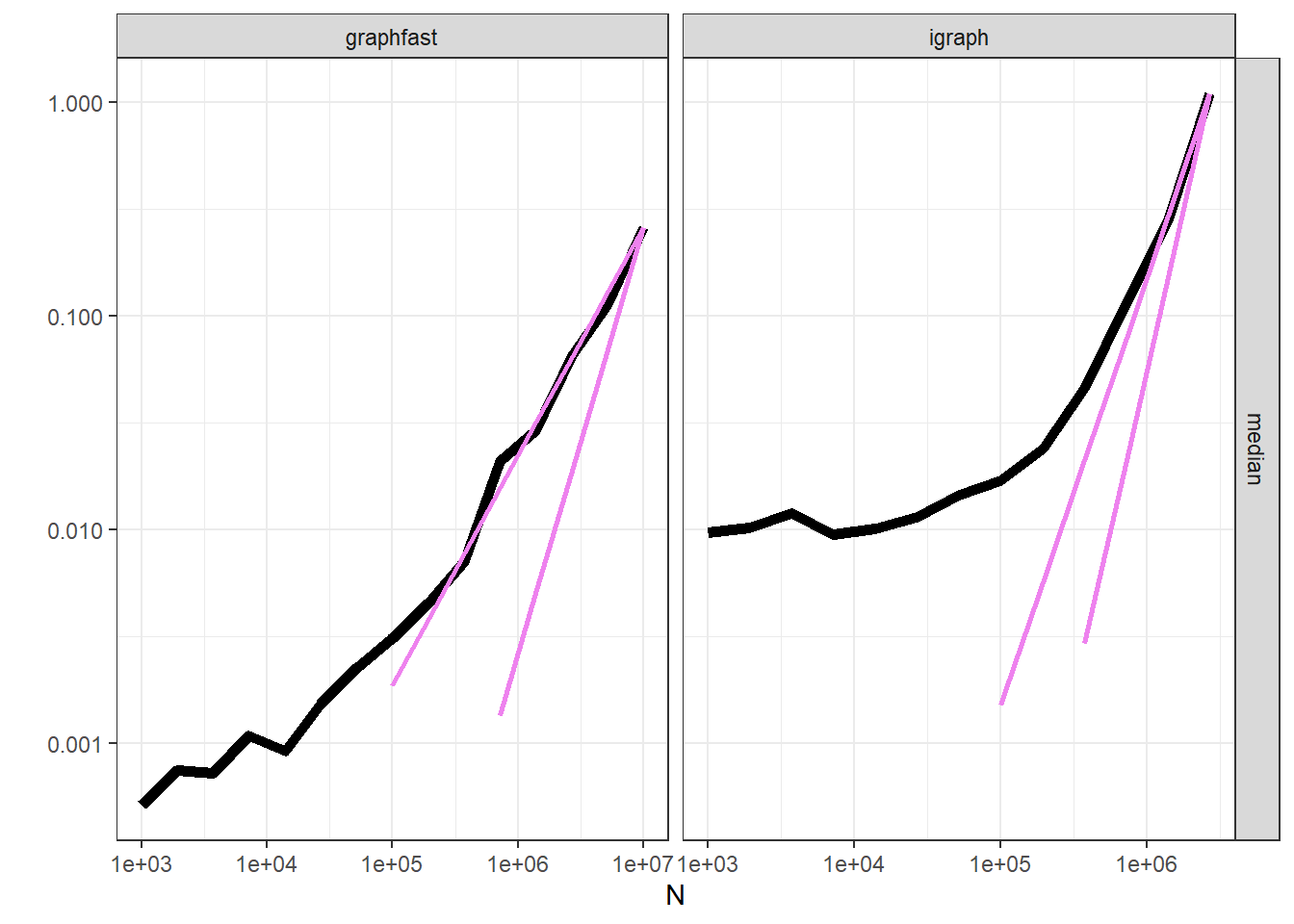
The tables above sample a handful of sizes. atime sweeps many more, timing each expression repeatedly per size and stopping once the median time crosses seconds.limit — so a slow contender doesn’t blow out the render — then fits the closest power-law/log/exponential reference curve to each series.
atime_result <- atime::atime(N =unique(as.integer(10^seq(3, 7, length.out =15))),setup = { edges <-make_graph(N) n_nodes <-max(edges) },seconds.limit =1,times =3,graphfast =find_connected_components(edges, n_nodes = n_nodes, compress =TRUE),igraph = igraph::components(igraph::graph_from_edgelist(edges, directed =FALSE)))# atime also measures memory via R's allocator (Rprofmem), but that only sees# memory allocated through R's own heap. igraph's graph structures are# allocated with raw malloc() inside its C library, invisible to that# tracker — so an atime memory comparison here would understate igraph and# can't be trusted. Time is unaffected by that blind spot, so we keep only# the time series here; real peak memory is measured separately below.atime_result$unit.col.vec <-"median"atime_refs <- atime::references_best(atime_result)plot(atime_refs)
Both curves are consistent with linear growth in edge count; the lines never cross — graphfast’s constant factor stays smaller across the whole range, and it keeps going to sizes where igraph has already crossed the time budget.
4.7 Varying the graph shape
Runtime is not just a function of edge count; structure matters. The sweep below holds the edge count fixed and varies sparsity (edges per node), measured live.
Sparsity — many small components (few edges per node) vs. one giant component (dense). Union–Find cost is dominated by the number of union calls (= edges) either way, but cache behaviour differs.
Component count — the relabelling pass is O(n_nodes); graphs with huge node spaces pay more there.
Query depth (shortest paths) — distant or unreachable pairs explore more of the graph; use max_distance to bound it.
4.8 Memory
graphfast’s connected-components memory is essentially:
so ~12 bytes per node plus the input. For sparse/large id spaces, prefer find_connected_components_safe(), which remaps ids so the arrays are sized by the number of distinct nodes, not the maximum id — the function reports the memory it saved in $memory_info. No adjacency matrix is ever formed, which is what makes 100M-edge graphs tractable on commodity hardware.
4.8.1 Measured peak memory
R-level memory profilers (Rprofmem, bench::bench_memory, and therefore atime’s memory metric) only see allocations made through R’s own heap. They miss memory a compiled library allocates itself with malloc()/calloc() — which is exactly how igraph’s C core manages its graph structures. Using one of those tools to compare graphfast against igraph would silently understate igraph’s real usage.
To get a number that’s actually comparable, each run below executes in its own fresh OS process — one package, one size, nothing else loaded — and reads back the peak working set the operating system recorded for that process (Windows’ PeakWorkingSetSize, via the ps package). That figure reflects everything the process touched, regardless of which allocator made the call.
This includes the cost of generating the graph itself (sampling, filtering self-loops) and R’s own baseline footprint — the same for both packages at a given size — so the difference between columns is the fair comparison, not the absolute numbers. igraph’s peak is consistently higher because building a full graph object (vertex table, attribute storage, internal adjacency structures) costs more than the union–find arrays graphfast works with directly.
4.9 Reproducing
# Install comparison packages as neededinstall.packages(c("igraph", "microbenchmark"))# The benchmark ships with the installed package — no need to clone the repo.# Runs 1e5, 1e6, 1e7 edges by default.source(system.file("benchmark.R", package ="graphfast"))# The scaling-behaviour and peak-memory sections on this page additionally use:install.packages(c("atime", "ggplot2", "ps"))
To regenerate the tables on this page, just re-render the book — the chunks above run automatically. Edit the sizes vector in the harness to push to 100M+ (and note your CPU, RAM, OS, R version, and threading, so the figures are comparable).